Ocr To Rag For Tables
OCR & RAG over tables
In order to have a high-performance RAG pipeline, source documents need to be properly processed and embedded. If not, the correct documents are not retrieved, and the answers can be wildly inaccurate. In this post, I look at tables inside PDFs. I discuss some of the challenges of performing OCR with Vision-language (VLMs) foundational models today, and show how adding the context to a table can yield ~40% more accurate answers compared to not adding the context.
Building a RAG over academic papers
Academic papers can have complex layouts (i.e. think multiple columns, nonlinear reading order), and in some research areas, such as STEM fields, multimodal data such as tables and charts are very prevalent. Everybody wants to have accurate answers in a RAG search. I would argue that getting accurate answers from a RAG search in an academic context (which could include medical applications for example) is perhaps more important than in most other areas. Not to mention that it is somewhat disappointing to create a RAG search over high-quality peer-reviewed research that might have taken years and a whole team to come by, so that the RAG pipeline then provides a wrong answer to a simple question.
Being able to quickly verify and find the sources of the answers is also an important requirement. Let’s say I’m a researcher conducting a literature review. If the RAG pipeline were to give me an answer and provide a whole pdf as a source, I might as well just decide to read the pdf in the first place. To be easily verifiable, the RAG pipeline needs to show the smallest snippet of text containing the information needed to answer a specific question: if it’s a table, show the table and its location, so a researcher can then easily verify it by looking at the table or finding it in the original document, if more context is needed.
Where VLMs struggle today with OCR
Academic papers can be found in a variety of formats, including structured formats like XML or LaTex. However, PDF is still very prevalent, specially for older research that was produced before digital copies were the norm. A PDF is a complex format that is not easily readable by a machine. In some cases, it’s just an image from a scanned document, and other times it’s a complex data structure. Even when the text is available, it won’t necessarily have a machine-readable representation of certain data structures like tables or formulas.
As an example, if you take Table 2 from this pdf, the text in the “text layer” looks like this:
Short-form
Closed-set
Long-form generations (with citations)
PopQA
TQA
Pub
ARC
Bio
ASQA
LM
(acc)
(acc)
(acc)
(acc)
(FS)
(em)
(rg)
(mau)
(pre)
(rec)
LMs with proprietary data
Llama2-c13B

[...]

Our SELF-RAG 13B
55.8
69.3
74.5
73.1
80.2
31.7
37.0
71.6
70.3
71.3
5
RESULTS AND ANALYSIS
It’s difficult to see what the column names and rows are. It’s also difficult to see where the table begins and where it ends. The number 5 at the end is the next section number (5. Results and Analysis) and not part of the table.
This is why there needs to be a processing step that turns a PDF into a more machine-friendly format before any searching can take place. This step is called OCR (Optical character recognition). There are many ways of performing OCR today with varying levels of success. Recent research found that vision-language multimodal foundational models (VLMs) that can handle both images and text provided a competitive method which often achieved best results (see OHR Bench paper).
Today’s VLMs can perform OCR on PDFs by converting them to the markdown format. In the example above, the same table in markdown looks like this:
| LM | **Short-form** PopQA (acc) | **Short-form** TQA (acc) | **Closed-set** Pub (acc) | **Closed-set** ARC (acc) | **Long-form** Bio (FS) | **ASQA** (em) | **ASQA** (rg) | **ASQA** (mau) | **ASQA** (pre) | **ASQA** (rec) |
|---|:--:|:--:|:--:|:--:|:--:|:--:|:--:|:--:|:--:|:--:|
| **LMs with proprietary data** |  |  |  |  |  |  |  |  |  |  |
| Llama2-C13B | 20.0 | 59.3 | 49.4 | 38.4 | 55.9 | 22.4 | 29.6 | 28.6 | — | — |
| Ret-Llama2-C13B | 51.8 | 59.8 | 52.1 | 37.9 | 79.9 | 32.8 | 34.8 | 43.8 | 19.8 | 36.1 |
| ChatGPT | 29.3 | 74.3 | 70.1 | 75.3 | 71.8 | 35.3 | 36.2 | 68.8 | — | — |
| Ret-ChatGPT | 50.8 | 65.7 | 54.7 | 75.3 | — | 40.7 | 39.9 | 79.7 | 65.1 | 76.6 |
| Perplexity.ai | — | — | — | — | 71.2 | — | — | — | — | — |
| **Baselines without retrieval** |  |  |  |  |  |  |  |  |  |  |
| Llama2-7B | 14.7 | 30.5 | 34.2 | 21.8 | 44.5 | 7.9 | 15.3 | 19.0 | — | — |
| Alpaca-7B | 23.6 | 54.5 | 49.8 | 45.0 | 45.8 | 18.8 | 29.4 | 61.7 | — | — |
| Llama2-13B | 14.7 | 38.5 | 29.4 | 29.4 | 53.4 | 7.2 | 12.4 | 16.0 | — | — |
| Alpaca-13B | 24.4 | 61.3 | 55.5 | 54.9 | 50.2 | 22.9 | 32.0 | 70.6 | — | — |
| CoVE-65B* | — | — | — | — | 71.2 | — | — | — | — | — |
| **Baselines with retrieval** |  |  |  |  |  |  |  |  |  |  |
| Toolformer*-6B | — | 48.8 | — | — | — | — | — | — | — | — |
| Llama2-7B | 38.2 | 42.5 | 30.0 | 48.0 | 78.0 | 15.2 | 22.1 | 32.0 | 2.9 | 4.0 |
| Alpaca-7B | 46.7 | 64.1 | 40.2 | 48.0 | 76.6 | 30.9 | 33.3 | 57.9 | 5.5 | 7.2 |
| Llama2-FT-7B | 48.7 | 57.3 | 64.3 | 65.8 | 78.2 | 31.0 | 35.8 | 51.2 | 5.0 | 7.5 |
| SAIL*-7B | — | — | 69.2 | 48.4 | — | — | — | — | — | — |
| Llama2-13B | 45.7 | 47.0 | 30.2 | 26.0 | 77.5 | 16.3 | 20.5 | 24.7 | 2.3 | 3.6 |
| Alpaca-13B | 46.1 | 66.9 | 51.1 | 57.6 | 77.7 | 34.8 | 36.7 | 56.6 | 2.0 | 3.8 |
| **Our SELF-RAG 7B** | 54.9 | 66.4 | 72.4 | 67.3 | 81.2 | 30.0 | 35.7 | 74.3 | 66.9 | 67.8 |
| **Our SELF-RAG 13B** | 55.8 | 69.3 | 74.5 | 73.1 | 80.2 | 31.7 | 37.0 | 71.6 | 70.3 | 71.3 |
The format above is a lot more machine-friendly and can be easily parsed and extracted. However, even if VLMs can turn PDFs into useful markdown, they can still struggle sometimes, specially if the PDFs have complex layouts. As a fun experiment, ask a VLM, such as the latest GPT-5, to determine the reading order of a document with multiple columns. Here are some of the results when asking a state-of-the-art VLM to provide a visual path for the reading order of a paper (just for fun):
And:
I tried different VLM providers to test their OCR accuracy over the first half of 2025, as well as non-VLM based approaches. AI keeps evolving and will no doubt improve over time for specific end use-cases. However, at the time of writing this article, these were the three major issues I encountered that had an impact on the downstream processing:
> broken paragraph text due to footnotes and other layout components
Often, if there is a table or a footnote in the page, the flow of text in the markdown output would get interrupted, and the end result would be a “broken paragraph” like in the example below.
The markdown looks like this:
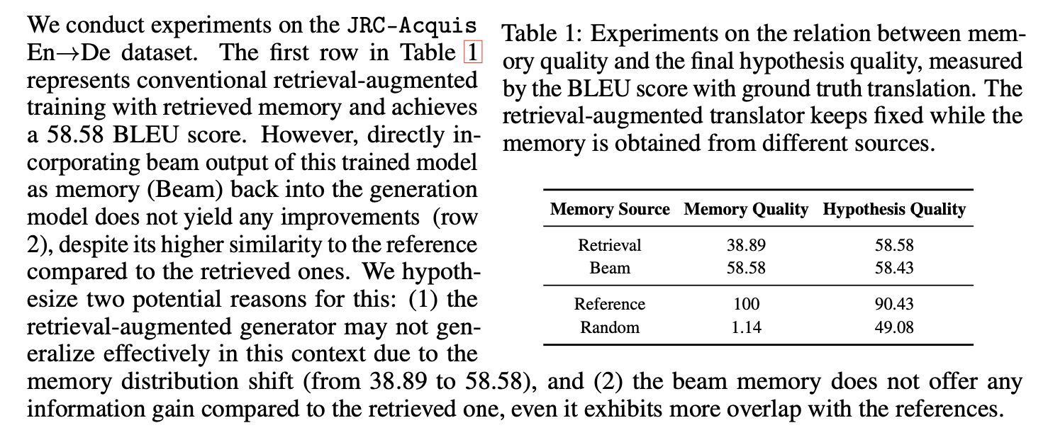
Furthermore, in-context machine translation has been shown to be effective for on-the-fly adaptation *[79]*. For dialogue response generation tasks, employing exemplar/template

---

| Memory Source | Memory Quality | Hypothesis Quality |
| --- | --- | --- |
| Retrieval | 38.89 | 58.58 |
| Beam | 58.58 | 58.43 |
| Reference | 100 | 90.43 |
| Random | 1.14 | 49.08 |

retrieval as an intermediate step has proven advantageous for generating informative responses *[89, 91, 6, 7]*.
The table caption is completely missing from the OCR.
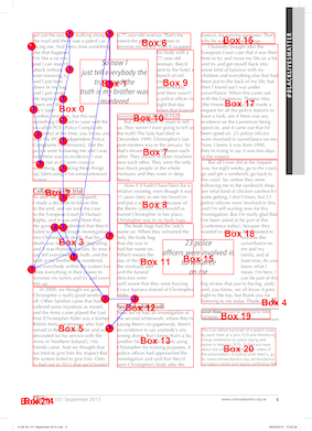
Another example of this can be found in the result by another provider: this time, Llamaparse and their state-of-the-art agentic OCR for scientific papers. I tested the preprint of this paper and there were many instances of broken paragraphs. This is an example of a footnote breaking the flow of text:
The markdown:
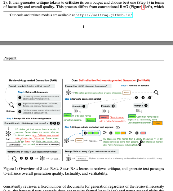
This process differs from conventional RAG (Figure 1 left), which

<sup>1</sup>Our code and trained models are available at https://selfrag.github.io/.
---

Preprint.

Retrieval-Augmented Generation (RAG)

Prompt How did US states get their names?
[...]
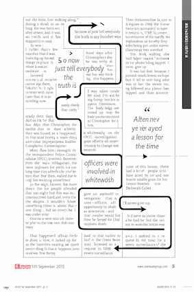
In the example above, the sentence at the end of the page is cut off in two, and the figure which contains text is not treated as such and is converted to text. The end result is very low-quality and not cheap at a cost of $4 (EU prices as of 09/25 for a 30-page document).
> wrong header levels
Many VLMs process pdfs on a page-by-page basis, and this sometimes means they get the hierarchy of the headings wrong or they’re not properly translated into markdown syntax. For example, I noticed that Gemini 2.5 pro model would sometimes use asterisks for headings, e.g. **Introduction** instead of the proper markdown syntax # Introduction.
In one of the papers OCR’d by Mistral, the hierarchy and numbering of the headers had many errors.
Mistral OCR extracted this header as # Induced and spontaneous mutation, putting it at the same level as the title of the paper and forgetting the 7.1 numbering. The headings of a specific section of a paper can carry important context about it, so it’s important to get this right.
> context of tables and figures not linked to the tables
VLMs are able to extract tables as markdown most of the time. However, there is no established way of associating a caption or label of a table to a specific table. So tables appear in the text separate from their captions and labels, making it very difficult for a RAG pipeline to use that context when answering questions about the table.
In the example below, I have two consecutive tables, making it non-trivial to know which caption goes with what table.
Just as a comparison, when using a XML-based format, the context of a table is typically encoded alongside the table. An example of a table defined in the JATS 1.4 looks like this:
<table-wrap id="t2" orientation="portrait" position="float">
 <label>Table II.</label>
 <caption>
  <p>Models to approximate the bound frequencies as waves
   in X→M (<inline-graphic id="g1" xlink:href="d1"/>: Rotational,
   <inline-graphic id="g2" xlink:href="d2"/>: Vibrate in <italic>y</italic>
   direction, <inline-graphic id="g3" xlink:href="d3"/>: Vibrate in
   <italic>x</italic> direction, <inline-graphic id="g4" xlink:href="d4"/>:
   Vibrate mainly in <italic>y</italic> direction including a small
   portion of vibration in <italic>x</italic> direction,
   <inline-graphic id="g5" xlink:href="d5"/>: Vibrate mainly in
   <italic>x</italic> direction including a small portion of vibration
   in <italic>y</italic> direction).</p>
 </caption>
 <table border="1">...</table>
</table-wrap>
Extracting the table content, its label and caption from the XML is straightforward.
As we can see, there are a lot of sources of error in the OCR process that could have an impact on the accuracy of a RAG pipeline down the line. Out of the errors identified above, I decided to focus initially on the problem of processing tables, and what happens if the context of a table (e.g. caption) is not included alongside the table.
A dataset for benchmarking
I used the dataset from the paper “OCR Hinders RAG: Evaluating the Cascading Impact of OCR on Retrieval-Augmented Generation”. This work had a github repository as well as a collection of pdfs and a dataset of questions and answers categorised by evidence source, i.e. whether the information was in a table, or in text, etc. I only sampled some of the pdfs and pairs of questions where the answer was in a table.
| Original dataset name | # of parsed academic pdfs | # question and answers using tables |
|---|---|---|
| OHR Bench | 49 | 314 |
An example of a question-answer pair:
{"ID": "57310e3c-3c2d-40f4-a3c1-969874ed4f14", "answer_form": "String", "answers": "Positive, Negative", "doc_type": "academic", "evidence_context": "SST-2 & \\begin{tabular}{l} Review: <S1> \\\\ Sentiment: <L> \\\\ Review: $<$ S> \\\\ Sentiment: \\end{tabular} & Positive, Negative", "evidence_page_no": 10, "evidence_source": "table", "full_pdf_path": "2305.14160v4.pdf", "questions": "What are the label words used for the SST-2 task in the demonstration templates?"}
The github repository also has code to compare the results of a RAG pipeline to the ground-truth answers. I used two of the metrics provided: the F1 and the exact match (EM) scores. When using exact match, the answers are first normalised and then compared to each other: if they’re the same, they receive a score of 1, if not it’s 0. The normalisation process is not always foolproof, specially for free-form answers. For example, the following pairs would get a score of 0:
| Ground-truth answer | LLM answer | EM score | F1 score |
|---|---|---|---|
| Near random accuracy | near random | 0 | 0.80 |
| Jajiya, Jagiya, Jisu, Jag, Jisutiya | Jajiya Jag Jagiya Jisutiya Jisu | 0 | 0.67 |
| × 2.99 | 2.99 | 0 | 0.67 |
| 4 | four | 0 | 0 |
The F1 score is between 0 and 1. It normalises both the ground-truth and the actual answer, tokenises them and compares their tokens. This scoring system is less strict than the exact match but also penalises some correct answers, as you can see from the examples in the table above.
The results
I ran a RAG pipeline over the dataset described before, with the only difference being how I processed the tables.
- Naive table chunking (
table without context): in this approach, I embedded the tables in their markdown format but did not try to add their caption or label to the same “chunk”. - Context-aware chunking (
table with context): the only difference with the above is that I tried to find the label and caption of each table and embedded both alongside the table contents in the same “chunk”.
Here are two examples, one where the chunk only contains the table:
| Year | Aurora | Giltner | Hampton | Hordville | Marquette | Phillips | Stockham |
| :-- | --: | --: | --: | --: | --: | --: | --: |
| 1890 | 1,862 | 195 | 430 | NA | 261 | NA | 211 |
| 1900 | 1,921 | 282 | 367 | NA | 210 | 186 | 169 |
| 1910 | 2,630 | 410 | 383 | NA | 290 | 274 | 189 |
| 1920 | 2,962 | 387 | 457 | 191 | 305 | 274 | 239 |
| 1930 | 2,715 | 355 | 369 | 175 | 318 | 221 | 211 |
| 1940 | 2,419 | 325 | 310 | 160 | 245 | 205 | 197 |
| 1950 | 2,455 | 284 | 289 | 116 | 218 | 190 | 82 |
| 1960 | 2,576 | 293 | 331 | 128 | 210 | 192 | 69 |
| 1970 | 3,180 | 408 | 387 | 147 | 239 | 341 | 65 |
| 1980 | 3,717 | 400 | 419 | 155 | 303 | 405 | 68 |
| 1990 | 3,810 | 367 | 432 | 164 | 281 | 316 | 64 |
| 2000 | 4,225 | 389 | 439 | 150 | 282 | 336 | 60 |
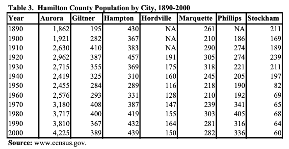
And another one where it has the label Table 3. and the caption:
Table 3. Hamilton County Population by City, 1890-2000
| Year | Aurora | Giltner | Hampton | Hordville | Marquette | Phillips | Stockham |
| :-- | --: | --: | --: | --: | --: | --: | --: |
| 1890 | 1,862 | 195 | 430 | NA | 261 | NA | 211 |
| 1900 | 1,921 | 282 | 367 | NA | 210 | 186 | 169 |
| 1910 | 2,630 | 410 | 383 | NA | 290 | 274 | 189 |
| 1920 | 2,962 | 387 | 457 | 191 | 305 | 274 | 239 |
| 1930 | 2,715 | 355 | 369 | 175 | 318 | 221 | 211 |
| 1940 | 2,419 | 325 | 310 | 160 | 245 | 205 | 197 |
| 1950 | 2,455 | 284 | 289 | 116 | 218 | 190 | 82 |
| 1960 | 2,576 | 293 | 331 | 128 | 210 | 192 | 69 |
| 1970 | 3,180 | 408 | 387 | 147 | 239 | 341 | 65 |
| 1980 | 3,717 | 400 | 419 | 155 | 303 | 405 | 68 |
| 1990 | 3,810 | 367 | 432 | 164 | 281 | 316 | 64 |
| 2000 | 4,225 | 389 | 439 | 150 | 282 | 336 | 60 |
For the rest of the pipeline, I tried to keep it as similar as possible to the initial paper by using the same embedding model (bge-m3) and same top_k parameter of 2.
These are the results:
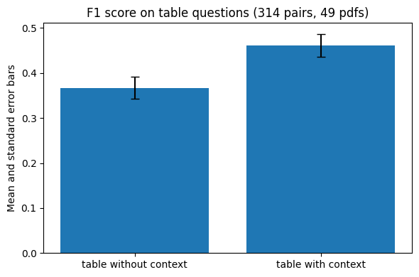
Naive table chunking (table without context) |
Context-aware chunking (table with context) |
|
|---|---|---|
| F1 metric | 0.37 (0.32 - 0.42) | 0.46 (0.41 - 0.51) |
| EM metric | 0.27 (0.22 - 0.32) | 0.36 (0.31 - 0.42) |
In practical terms, what does it mean? I estimated this manually by checking a sample of answers where the table with context method achieved a better F1 score than the table without context one. What it means in real terms: we can answer 38% more questions accurately using the context of the table. The rest of the time the answers are either plain wrong or unspecified.
Some examples of questions that could not be answered due to missing context:
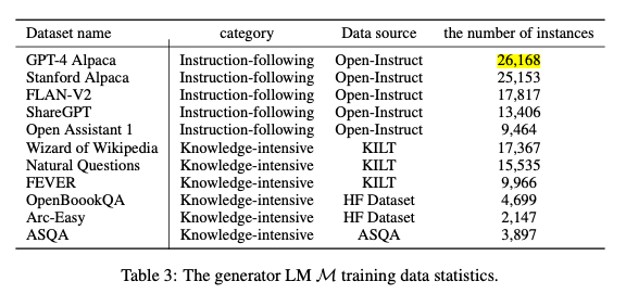
- In table 3 from this paper, to the question “What is the number of instances in the GPT-4 Alpaca dataset used for training the generator LM?”, the RAG pipeline without table context could not answer the question (i.e. “Not specified”). As you can see from the below image, the table does not have a lot of text so it needs the caption to link it to some important concepts contained in the question, such as “generator LM” or “training”.
- This is another example where the caption is needed to understand what the table represents. In this scenario, the
table without contextmethod did not manage to locate the correct table when asked a question about it, and tried to answer the question without using the context provided, which can lead to misleading answers that sound correct. Without the caption in the table, it’s hard to interpret what the numbers inside the table represent.
- Sometimes the captions are included as cells in the tables. However, the OCR’d result did not always include the caption inside the table.
This is how the table looks like:
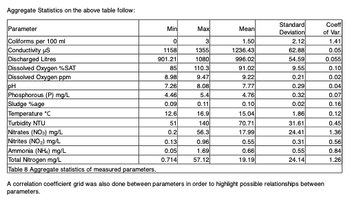
This is how Mistral parsed it:
Aggregate Statistics on the above table follow:

| Parameter | Min | Max | Mean | Standard <br> Deviation | Coeff <br> of Var. |
| :-- | --: | --: | --: | --: | --: |
| Coliforms per 100 ml | 0 | 3 | 1.50 | 2.12 | 1.41 |
| Conductivity $\mu \mathrm{S}$ | 1158 | 1355 | 1236.43 | 62.88 | 0.05 |
| Discharged Litres | 901.21 | 1080 | 996.02 | 54.59 | 0.055 |
| Dissolved Oxygen \%SAT | 85 | 110.3 | 91.02 | 9.55 | 0.10 |
| Dissolved Oxygen ppm | 8.98 | 9.47 | 9.22 | 0.21 | 0.02 |
| pH | 7.26 | 8.08 | 7.77 | 0.29 | 0.04 |
| Phosphorous (P) mg/L | 4.46 | 5.4 | 4.76 | 0.32 | 0.07 |
| Sludge \%age | 0.09 | 0.11 | 0.10 | 0.02 | 0.16 |
| Temperature ${ }^{\circ} \mathrm{C}$ | 12.6 | 16.9 | 15.04 | 1.86 | 0.12 |
| Turbidity NTU | 51 | 140 | 70.71 | 31.61 | 0.45 |
| Nitrates $\left(\mathrm{NO}_{3}\right) \mathrm{mg} / \mathrm{L}$ | 0.2 | 56.3 | 17.99 | 24.41 | 1.36 |
| Nitrites $\left(\mathrm{NO}_{2}\right) \mathrm{mg} / \mathrm{L}$ | 0.13 | 0.96 | 0.55 | 0.31 | 0.56 |
| Ammonia $\left(\mathrm{NH}_{4}\right) \mathrm{mg} / \mathrm{L}$ | 0.05 | 1.69 | 0.66 | 0.55 | 0.84 |
| Total Nitrogen mg/L | 0.714 | 57.12 | 19.19 | 24.14 | 1.26 |

Table 8 Aggregate statistics of measured parameters.
A correlation coefficient grid was also done between parameters in order to highlight possible relationships between parameters.
As you can see the caption is not included inside the table.
Conclusion
In this post, I created a benchmark for RAG accuracy on tables to compare different approaches. I am aware that there are many types of RAG pipelines and chunking techniques, and have not tried to do any further optimisation yet, but I’m planning to do this in the future.
The output of state-of-the-art VLM OCR models still needs a lot of processing before it can achieve reasonable RAG accuracy on PDFs with complex layouts. The tl-dr is: if you use naive table processing, you will end up with a very low-quality RAG search application over your data.